Monte Carlo Recovery of a Known Structure with CFA-Boosting
Source:R/simulate_cfa_recovery.R
simulate_cfa_recovery.RdThe confirmatory counterpart of simulate_recovery. Data are
simulated from a known population, a simple structure model over every item
is handed to cfa_boosting, and the question is how often the
pipeline removes the items that deserve removal and only those.
Usage
simulate_cfa_recovery(
  n = 500,
  loading = 0.65,
  items_per_factor = 5,
  n_factors = 3,
  phi = 0.3,
  n_cross = 1,
  cross_loading = 0.4,
  n_low = 1,
  low_loading = 0.2,
  n_categories = 5,
  skew = c("symmetric", "skewed"),
  n_reps = 100,
  seed = NULL,
  verbose = TRUE,
  n_cores = 1,
  timeout = 120,
  ...
)

# S3 method for class 'simulate_cfa_recovery'
print(x, ...)
Arguments
- n
Sample size(s). Vector values are crossed into conditions. Default 500.
- loading
Population loading(s) of the good items. Default 0.65.
- items_per_factor
Number of good items per factor. Default 5.
- n_factors
Number of factors in the population model. Default 3.
- phi
Interfactor correlation. Default 0.30.
- n_cross
Number of cross-loading items added to the pool (they load
cross_loadingon factors 1 and 2). Default 1.- cross_loading
Loading of the cross-loading items on both factors. Default 0.40.
- n_low
Number of weak items added to the pool. Default 1.
- low_loading
Loading of the weak items. Default 0.20.
- n_categories
Number of ordered response categories. Default 5.
- skew
Category threshold shape:
"symmetric"(default) or"skewed".- n_reps
Replications per condition. Default 100.
- seed
Optional integer seed for reproducibility; NULL (default) leaves the RNG untouched.
- verbose
Print progress per condition. Default
TRUE.- n_cores
Number of worker processes used to fit the replications of a condition. Default 1 (sequential). A crossed design is hundreds of
efa_boosting()runs, so this is usually the difference between minutes and hours;parallel::detectCores() - 1is a practical choice. The datasets are always generated sequentially fromseed, so results do not depend on the number of cores.- timeout
Seconds allowed per replication. Default 120;
NULLremoves the cap. A single pathological dataset can otherwise grind for many minutes and stall the condition it belongs to. A capped replication is recorded withstop_reason = "timeout". Needs theR.utilspackage.- ...
Ignored.
- x
A
simulate_cfa_recoveryobject.
Value
An object of class simulate_cfa_recovery: a list with
summary (one row per condition), replications,
conditions, population, model (the syntax handed to
the pipeline) and call.
Details
The question is not the same one the exploratory simulation asks, and the
difference is not cosmetic. In simulate_recovery the structure
is discovered, so recovery means every retained item landed on its true
factor. Here the structure is imposed by the researcher, so the assignment
cannot be wrong by construction and what is at stake is the item selection:
the specified model deliberately includes the contaminated items, and a
pipeline that works removes them without taking good items with them.
Two further quantities are worth watching. covs_added counts the
residual covariances the pipeline introduced: the population has none, so
every one of them is a false positive, which is the modification index
objection of MacCallum, Roznowski and Necowitz (1992) turned into a number.
And exact is deliberately strict, requiring the removed set to equal
the contaminated set exactly, because sensitivity and specificity can both
look respectable while no single replication got the answer right.
The cross loading item is specified on the first factor and the weak item as well, which is what a researcher would do when writing the model without knowing which items are faulty.
Examples
# \donttest{
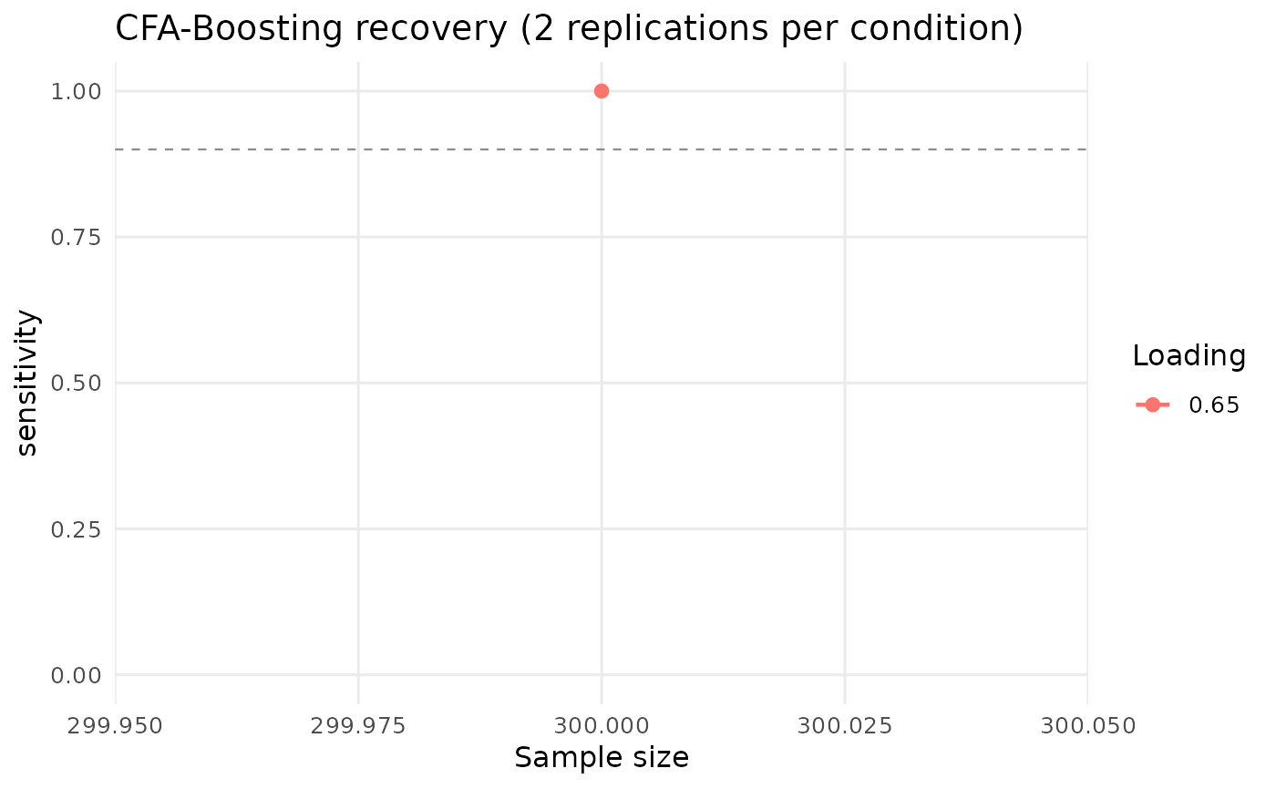
sim <- simulate_cfa_recovery(n = 300, n_reps = 2, seed = 1)
#> Condition 1/1: N=300, lambda=0.65, items/factor=5 (17 items total)
#>
[ ] 0% (0/2) elapsed 0s left ~?
[============= ] 50% (1/2) elapsed 3s left ~3s
[==========================] 100% (2/2) elapsed 6s left ~0s
sim
#>
#> CFA-Boosting recovery simulation
#> --------------------------------------------------------------------
#> 1 condition(s) x 2 replications
#> Population: 3 factors, roles: cross=1, good=15, low=1
#>
#> n loading items_per_factor n_reps convergence_rate exact_rate sensitivity
#> 300 0.65 5 2 1 1 1
#> specificity mean_retained mean_covs_added mean_rmsea
#> 1 15 0 0.012
#>
#> exact_rate = the removed set equals the contaminated set, item for item.
#> sensitivity = contaminated items removed; specificity = good items kept.
#> mean_covs_added = residual covariances added; the population has none,
#> so anything above zero is capitalization on chance.
plot(sim, metric = "sensitivity")
#> `geom_line()`: Each group consists of only one observation.
#> ℹ Do you need to adjust the group aesthetic?
 # }